In this section, you will continue with the Lab1_binary directory from the introduction. You can also re-download a copy of the desired Lab1_binary MESA work directory, but make sure pgbinary_flag is set to true in inlist_project as we did in the introduction.
Lab1 - Modeling a star through envelope stripping
Science goal
In this lab, we will look at how stars stripped by binary interactions evolve compared to their single star counterparts. We will look at how the appearance (e.g. luminosity, temperature), structure (e.g. core mass) of the donor star changes depending on the binary orbital parameters and mass transfer efficiency. These properties are very important when we compare stellar models to observed pre-supernova progenitors.
Bonus goal
If you’d like to prepare for Lab3, you can start running a simulation with both stars and leave it running over lunch.
The evolution of the primary star
Assume that we have a binary star system where the components are close enough to undergo Roche Lobe overflow (RLOF) from the inner L1 Lagrangian point. Additionally, assume that both components do not have the same mass so that the evolution of one star slightly lags the other star. In the lab, we would like to explore how the primary - more massive - star evolves in such a binary.
Since here we are primarily interested in the evolution of the primary, to save some computation time we are going to approximate the secondary as a point mass. In other words, we are not going to model the evolution of the secondary. Then, later in Lab3, we will switch to treating the primary as a point mass and focus on evolving the secondary mass gainer (accretor).
Let’s begin by using the downloaded Lab1_binary directory from the introduction. We will begin by modeling this system as a star + point mass. To do this, open inlist_project and make sure to set evolve_both_stars = .false..
In the &binary_controls, you should see the following lines:
   m1 = 15d0  ! donor mass in Msun
   m2 = 12d0 ! companion mass in Msun
   initial_period_in_days = 6d0
A range of parameters to adjust the mass transfer efficiency are also available in inlist_project. Below is an example of a fully conservative mass transfer scheme where all the mass lost by the primary is assumed to be accreted onto the secondary ($\dot{M}_2=-\dot{M}_1$).
   ! Mass transfer efficiency controls
   mass_transfer_alpha = 0d0      ! fraction of mass lost from the vicinity of donor as fast wind
   mass_transfer_beta = 0d0     ! fraction of mass lost from the vicinity of accretor as fast wind
   mass_transfer_delta = 0d0    ! fraction of mass lost from circumbinary coplanar toroid
   mass_transfer_gamma = 0d0    ! radius of the circumbinary coplanar toroid is ``gamma**2 * orbital_separation``
For non-conservative mass transfer, part of the mass that is transferred to the accretor escapes the system ($\dot{M}_2=-(1-\alpha-\beta-\delta)\dot{M}_1$). The lost mass can take away some angular momentum from the binary, and the amount of angular momentum it takes away depends on the details of the mass transfer flow. Each of the mass transfer parameters corresponds to a different angular momentum loss mode, as described in the comments. Here, we will assume that the non-accreted mass takes away the specific angular momentum of the accretor (Jeans mode mass loss). For example, if half of the transferred mass is lost from the system, we set the parameters like this
mass_transfer_beta = 0.5d0 ! fraction of mass lost from the vicinity of accretor as fast wind
Now, let’s explore the different types of mass transfer and the impact of nonconservative mass transfer on the evolution of our binary system.
For this lab we will keep the primary and companion/accretor mass fixed at m1 = 15d0 and m2 = 12d0, do not adjust these masses. We will explore the effect of different masses and mass ratios later on in Lab2. In this lab we will explore the binary evolution of our system with varying periods by modifying initial_period_in_days, and the impact of adopting nonconservative mass transfer by adopting a different value for $\beta$. Each person at your table will run one of the following four models shown in the table below, and you will compare and discuss your results with one another.
| Case | Donor Mass ($M_{\odot}$) | Accretor Mass (M$_\odot$) | Period (days) | $\beta$ |
|---|---|---|---|---|
| 1 | 15 | 12 | 4 | 0 |
| 2 | 15 | 12 | 15 | 0 |
| 3 | 15 | 12 | 200 | 0 |
| 4 | 15 | 12 | 15 | 0.5 |
|
|
|---|
| Now choose a value for the initial period and $\beta$ of the binary system from this table. |
For solar metallicity stars, it is known that mass transfer processes will strip most of the hydrogen envelope over relatively short timescales. However, the computational cost ramps up as the remaining envelope mass decreases, so we could end up spending most of our computation time trying to strip off the last bit of envelope, even though it may not be long in physical time. In the first half of this lab, we will focus on examining the stability and timescale of mass transfer, so let’s apply a stopping condition to terminate the calculation before the computation slows down.
|
|
|---|
| Try to apply a stopping condition so that the calculation finishes when 80% of the donor’s envelope is lost. See MESA &controls documentation: When to stop. |
|
|
|---|
This can be done by setting a stopping condition in inlist1. |
Don’t forget to uncomment the mass transfer parameters by deleting the ! in front of them. |
Answers: Example code
Add this to &controls in inlist1
envelope_fraction_left_limit = 0.2
Now, let’s run the model. We need to execute the below commands in the terminal to compile our run_binary_extras.f90 file and run the calculation.
$ ./mk
$ ./rn
The model should take roughly 4 minutes to run on a 4 core machine, you can use this time to inspect and discuss differences between your models and those of the others at your table.
When your model has finished running, try to make a movie of your &pgbinary diagram so you can watch the movie instead of re-running your MESA model. In your Lab1_binary directory you can execute the images_to_movie command to convert your saved &pgbinary pngs into a movie. Here is an example that produces a .mp4 movie named movie.mp4.
$ images_to_movie "png/*.png" movie.mp4
|
|
|---|
| If the command doesn’t work, make sure to update your MESA SDK. |
Answers: An example pgbinary produced from the case 1 in the table above
Now that you have created a wonderful &pgbinary movie, let’s use this movie in conjuction with our terminal output from our run to answer the following questions!
|
|
|---|
If you are having issues generating a pgbinary movie, we have provided precomputed &pgbinary movies for all the runs available for download here. |
Below are some questions to discuss at your table and answer while your model evolves
|
|
|---|
| 1. What type of mass transfer does your system undergo? Case A, B, C? |
| 2. Is the mass transfer in your system stable or unstable? |
| 3. What is the mass transfer timescale (e.g. $\tau_\mathrm{mt}\equiv |M_1/\dot{M}_1|$)? |
What are the different types of mass transfer?
Mass transfer in binary systems are often classified based on which burning stage the donor star is in. This is because stars have very different structures depending on the burning stage and therefore respond to mass loss in completely different ways.
- Case A mass transfer
- Mass transfer from a core hydrogen burning star (main sequence star).
- Case B mass transfer
- Mass transfer from a core hydrogen depleted star (post-main sequence star).
- Case C mass transfer
- Mass transfer from a core helium depleted star.
We sometimes combine the different types if multiple mass transfer phases occur in the same system. For example, if Case A mass transfer is followed by Case B mass transfer, we call it Case AB mass transfer.
How do we know which type of mass transfer occurs? This can be done by simply comparing the size of the star during various burning stages to the size of its Roche lobe.
The Roche lobe size can be estimated with the following formula
\[\frac{R_\mathrm{rl}}{a} = \frac{0.49q^{2/3}}{0.6q^{2/3}+\ln{(1+q^{1/3})}}\equiv f(q)\]Here, $R_\mathrm{rl}$ is the volume equivalent Roche lobe radius of the donor, $a$ is the orbital semimajor axis and $q\equiv M_\mathrm{d}/M_\mathrm{a}$ is the mass ratio of the donor to accretor. Mass transfer occurs when the stellar radius exceeds the Roche lobe radius $R_\mathrm{d}>R_\mathrm{rl}$.
|
|
|---|
| Calculate the orbital period ranges for Case A/B/C mass transfer for a 15+12$M_\odot$ binary. |
The radius evolution of our 15$M_\odot$ star looks like this:
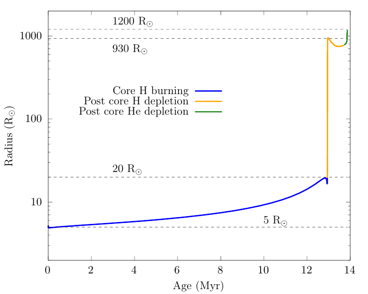
Radius evolution of a 15 M$_\odot$ star
Different colours indicate which burning stage the star is in. The dashed lines mark the radii of the star at ZAMS and the maximum extent during each burning stage.
Answers
If the donor star engages in mass transfer at a given radius $R$, the orbital separation needs to be $a=R/f(q)$. The orbital period of a binary is given by Kepler's law $$ P_\mathrm{orb}=2\pi\sqrt{\frac{a^3}{G(M_1+M_2)}}. $$- Case A: $1~\mathrm{d}\lesssim P_\mathrm{orb}\lesssim7.9~\mathrm{d}$
- Case B: $7.9~\mathrm{d}\lesssim P_\mathrm{orb}\lesssim2517~\mathrm{d}$
- Case C: $2517~\mathrm{d}\lesssim P_\mathrm{orb}\lesssim3689~\mathrm{d}$
Bonus 1: Evolving through the whole mass transfer phase
Now that we know all of our models were either case A or case B mass transfer, let’s extend the our stopping condition further until core-Carbon depletion. This will allow us to determine whether our models undergo a second mass transfer phase, and whether or not they end their lives a Blue, Yellow, or Red Supergiant (BSG,YSG,RSG).
First, remove the stopping condition we applied earlier. Then in run_star_extras.f90, let’s add a new stopping condition so that our model terminates when the primary reaches core Carbon depletion. Let’s terminate the model when $X(^{12}\mathrm{C})\leq10^{-4}$:
Note that just adding a control like the following will not work for all cases. But why?
      xa_central_lower_limit_species(1) = 'c12'
      xa_central_lower_limit(1) = 1d-4
This is because most of the initial $^{12}\textrm{C}$ present at ZAMS is converted into $^{14}\textrm{N}$ via the CNO cycle during core-Hydrogen burning. The $^{12}\textrm{C}$ present in the core at the onset of Carbon burning is produced via the $3\alpha$ and $^{12}\mathrm{C}(\alpha,\gamma)^{16}\mathrm{O}$ reactions during core-Helium burning. To prevent our models from prematurely terminating, we need to add a custom stopping condition in our run_star_extras.f90.
|
|
|---|
| Add a custom stopping condition that will terminate your model when the central mass fractions $X(^{12}\mathrm{C})\leq10^{-4}$ and $X(^{4}\mathrm{He})\leq10^{-4}$ are both true. |
|
|
|---|
Specifically, you’re looking to modify the extras_finish_step function in run_star_extras.f90. |
Answers: Example c12 stopping condition
integer function extras_finish_step(id)
   use chem_def , only: ihe4, ic12
   integer, intent(in) :: id
   integer :: ierr
   type (star_info), pointer :: s
   ierr = 0
   call star_ptr(id, s, ierr)
   if (ierr /= 0) return
   extras_finish_step = keep_going

   if (s% xa(s% net_iso(ic12),s% nz) < 1d-4 .and. s% xa(s% net_iso(ihe4),s% nz) < 1d-4) then
      extras_finish_step = terminate
      write(*,*) 'Reached Core Carbon depletion, Model finished evolution.'
   end if

end function extras_finish_step
When you’re finished modifying the run_star_extras.f90 file, be sure to check that your code compiles by running the following and terminating your model after a few timesteps.
$ ./clean
$ ./mk
Now that we’ve added our new stopping condition, you can save yourself some computation time by restarting your binary mass transfer model from the photo created at the end of your previous run. This can be done by executing the following example command in the terminal for a model that terminated at timestep 353.
$ ./re x000353
Again, you can make &pgbinary movie of your run and use it with your terminal output to answer the following questions!
|
|
|---|
If you are having issues generating a pgbinary movie, we have provided precomputed &pgbinary movies for all the runs available for download here. |
Answers: An example pgbinary produced from the case 1 in the table above
|
|
|---|
| 1. How much of the envelope has the donor lost? |
| 2. Is the appearance of the donor (luminosity and temperature) different from what you would expect for a normal core He depleted star? |
| 3. Is there another mass transfer phase following the first one (Case AB/BB)? |
| 4. What do your supernova progenitor look like, is it a Blue, Yellow, or Red Supergiant? |
| 5. What kind of observational supernova would the primary star explode as? |
Here are some rough characteristic effective temperatures for massive stars (adopted from Drout et al. 2009):
Blue Supergiant (BSG): > 7,500 K
Yellow Supergiant (YSG): 4,800 K – 7,500 K
Red Supergiant (RSG): < 4,800 K
Bonus 2: Evolving both stars
In Lab3, we will be exploring how the accretor star can evolve differently from single stars of the same mass. For this, we need to run the evolution with both stars without assuming the secondary star is a point source. This typically takes much more time than the point source case, so let’s keep a model running before you leave for lunch.
We’d like to save the final accretor_final.mod file from the accretor (secondary) for use in Lab3, so let’s remove all the stopping conditions we applied earlier. Then in inlist1, set a stopping condition such that the model terminates when the primary reaches core helium depletion. Let’s terminate the model when $X(^4\mathrm{He})\leq10^{-4}$:
We can do this by adding the following stopping condition in inlist1
      xa_central_lower_limit_species(1) = 'he4'
      xa_central_lower_limit(1) = 1d-4
Run the same model as you did in Lab1 but now with
evolve_both_stars = .true.
|
|
|---|
If you are having issues generating a pgbinary movie, we have provided precomputed &pgbinary movies for all the runs available for download here. |
You will now see both stars being evolved in the &pgbinary plots that looks like this.
Remember you’ll be using your accretor_final.mod from this bonus in Lab3, but don’t worry if you don’t get this far as we will provide a copy of accretor_final.mod for you if you run out of time before generating one yourself.
|
|
|---|
If you are having issues generating the accretor_final.mod file for Lab3, we have provided precomputed mod files available for download here. |